World-renowned, Microsoft Excel is one of the most popular and highly functional spreadsheet applications available. It has become a benchmark for students and professionals who need to organize, arrange, and manage critical data, including data entry and transportation.

If you don’t think you will need this vital Microsoft Office suite member as a tool in your kit during college, consider the fact that 82% of employers require Excel user skills or experience. Additionally, certified Excel skills can increase your earning potential by an average of 12%. According to Investopedia, professions in fields including finance and accounting, marketing and product management, human resource planning, and many more use Excel to manage their business better.

Whether you are starting your college career and have no experience with the Excel worksheet application, or you want to brush up on your existing skills, you’ll benefit from learning some tricks to minimize the number of clicks and maximize effectiveness with the following 30 awesome Microsoft Excel tips and tricks:

1. HELPFUL KEYBOARD SHORTCUTS

Keyboard shortcuts might take a little time to memorize, or you can peek at special cheat sheets for reference until they become second nature, but once you commit them to memory, they are fantastic time savers.

You execute most shortcuts using the Control (“Ctrl”) key and a corresponding letter that represents the action. Sometimes the assigned letter makes logical sense, such as O for opening an existing workbook. At other times, such as Z, for undoing your last action, you need to think outside the box a bit. With these keyboard shortcuts, click Ctrl and the intended letter simultaneously, hence the + sign.

Below are some essential shortcuts that allow you to do everything from creating a new workbook to cutting and pasting information from one cell to the next quickly and accurately.

2. QUICKLY DELETE BLANK CELLS

When you start reviewing your worksheet, you might notice one or more blank cells that you need to remove. You can delete blank cells in a few ways:

• Click on the range of cells you want to remove, select the Home tab, then under the Editing section, choose Find & Select before picking Go To Special.

• Once at Go To Special, select Blanks and OK to confirm.
• Go to the Home tab and in the Cells group, choose Delete.

3. ADD A DIAGONAL LINE TO A CELL

The border function comes in handy when you want to add a diagonal line inside a cell. Try this:

• Push the cell where you want to place a diagonal line.
• Right-click the cell to select Format Cells, and that dialog box will pop up.
• Choose Border at the top ribbon in the tabs at the top, then choose a diagonal line.
• Preview your diagonal line in the box.

4. SELECT ALL CELLS IN A SPREADSHEET

You can quickly perform this task by clicking the Select All button in the upper left-hand corner of the spreadsheet. Another quick and simple way to execute this task is to click CTRL+A.

5. COPY A FORMULA ACROSS ROWS OR DOWN COLUMNS

Here is a quick way to copy a formula down a row or column:

• Place your formula in the top cell.
• Choose the cell with that formula and hover your cursor over the small square at the lower right corner of the cell. This is called the Fill Handle. You will see a thick or bold cross-shape replace your standard cursor.
• Grab and drag the Fill Handle down the column or across the row, covering the cells where you want to copy the formula.

6. PRINT OPTIMIZATION

When you think of printing as a process, it becomes much simpler. Much of it is easily manageable. Start here to find your tools and options for print optimization:

• Click the File tab. (Figure 1)
• Select Print where you will then see a full preview of your document. (Figure 2)
• Use Settings to select preferences, such as the number of pages or to print on the front and back of the paper.

Figure 1

Figure 2

7. IMPORT A TABLE FROM THE WEB

Excel users sometimes need to insert or import a table from the web. Here are some steps to do that:

• Copy the URL.
• Select Data > Get & Transform > From Web.
• Click CTRL+V to paste the URL into the text box, then press OK.
• Use the Navigator pane under Display Options, then choose the Results table.
• You can preview the results in the pane to the right called Table View.
• Choose to Load your results through Power Query, which changes the data, loading it as an Excel table.

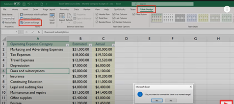
8. CONVERTING NUMBERS TO RANGES

Sometimes you might want to see only a range of numbers. Here’s how to do this task:

Select any spot in the table, then go to Table Design.
Under Tools, choose to Convert to Range.

Even better, you can use this shortcut where you click Table > Convert to Range.

9. FLASH FILL

Flash fill acts like autocorrect, detecting data patterns in your spreadsheets. Once Excel detects patterns, you’ll see the cells following as shaded. Just click Enter to accept the flash fill option.

10. FORMAT PAINTER

One of the most underused formatting features, Format Painter allows you to copy formatting from one cell or group of cells to another.

• Select the formatted cell you want to copy.
• Go to the Home tab and choose Format Painter.

• The cell’s border will turn into dashed lines, and your cursor will become a paintbrush.

• Click on the cell where you want to duplicate the formatting, and it will appear.

11. FONT COLOR WITH CUSTOM FORMATTING

You might want to assign meaning to font color as a shortcut, such as green for positive values and red for negative values. This tip is tricky, but here are the basics of getting started with it:

• Choose your cell and press CTRL+1 to open the Format Cells dialog box.
• Select Custom.
• Type in the necessary format code in the Type box, then click OK.

12. AUTOFORMAT

Simplify the formatting process with Excel’s handy AutoFormat option. Go to the Quick Access Toolbar drop-down, then choose the commands you need.

• Go to the Quick Access Toolbar drop-down and click More Commands.
• Click the Choose commands from drop-down and select All Commands.
• Choose AutoFormat, click Add then OK. This adds AutoFormat to the Quick Access Tool Bar.

To use AutoFormat, highlight the data you’d like to format, click AutoFormat and choose a style.

13. SELECT A NON-ADJACENT CELL

If you’re a mouse user, this task is simple enough. Click on the cell, then drag to include the other cells you want.

For keyboard users, it’s a little more complicated:

• Choose the cell you want to activate.
• Press F8 to the cell into Extend Selection mode, which you will see in the status bar.
• Use your arrow keys to go left, right, up, or down, choosing the appropriate non-adjacent cells.
• Hold Shift and F8 simultaneously, which allows you to Add or Remove Selection.

14. TOTAL A COLUMN OR A ROW

One of the best and quickest ways to total a row or column is by enabling the Total Row or Total Column option under the Design tab.

15. PIVOT TABLES

Pivot tables empower you to extract key data points from large sets of data.

To insert a pivot table.

• Click into a single cell inside the data set.
• On the Insert tab, in the Tables group, select Pivot Table.
• Select the relevant table or range, then click OK.

16. ADD MORE THAN ONE NEW ROW OR COLUMN

When you need another row or column, try the following:

• Choose the number of rows or columns you want to add, then right-click on them.
• Select Insert from the drop-down menu.

17. ADD BULLET POINTS

A simple trick for adding bullets to a cell is clicking the desired cell, then pressing ALT+7.

18. SHIFT BETWEEN DIFFERENT EXCEL FILES

You might think clicking back and forth between different files is complicated, but fortunately, it’s a quick and simple maneuver. Click CTRL+Tab or ALT+Tab.

19. USE TABLE CREATION TO PREVENT SHIFT

The best way to prevent row or column shift is to create a table with your data to prevent you from inadvertently inserting a cell that shifts the data.

20. USE THE IF EXCEL FORMULA TO AUTOMATE CERTAIN EXCEL FUNCTIONS

The IF function has become extremely popular and more widely used over the years, allowing you to make meaningful comparisons between a resulting value and the value you expected.

21. INSERT EXCEL DATA INTO WORD

There are many times when Excel and Word go hand-in-hand. You might find that you need to insert Excel data into Word documents more often than you would imagine, but data can often make your case to a professor or employer when the most effective text will not.

One quick way to add Excel data is by linking the worksheet into the document. Another way you can do it is by pushing CTRL+C or Command+C to copy the information. Next, paste it where you want in Word.

22. ADD DROP-DOWN MENUS

Another way to add efficiency in Excel is by creating drop-down menus by typing the entries you want into an Excel table. Even if you don’t have your items in a table, you can quickly achieve this task by selecting any cell in the range, and pressing CTRL+T. Next, select where you want the drop-down list, and press Data, then Data Validation. You’ll next see the Settings tab, then go to the Allow box, and click List. After that, select your range in the Source box. Finally, you check the In-cell dropdown box and click the Input Message tab.

23. HYPERLINK A CELL TO A WEBSITE

Fortunately, this popular and extremely useful task is straightforward. Click on the cell and go to the Insert tab, then click Link and add the URL in the address bar.

24. ADD CHECKBOXES

Form controls like checkboxes make it easier to enter data uniformly.

First, go to the Developer tab on your Ribbon. Click Insert, then make a selection.

25. COUNTIF FUNCTION

COUNTIF is a statistical function that lets you count the number of cells that align with certain Criteria, such as the number of times a city is cited in a customer list. Keep in mind that Criteria aren’t case sensitive, meaning you will see every instance when conducting a COUNTIF query.

Basically, COUNTIF says:

• =COUNTIF(Where do you want to look?, What do you want to look for?)

For Example:

• =COUNTIF(A2:A35, “New York”)
• =COUNTIF(A2:A35,A4)

26. INDEX AND MATCH FORMULAS TO PULL DATA FROM HORIZONTAL COLUMNS

The Trump Excel website recommends thinking of the INDEX & MATCH FUNCTIONS acting as GPS satellites. Essentially, these functions create coordinates that help you navigate your spreadsheet.

Here is a great example from Ablebits:

27. VLOOKUP FUNCTION TO PULL DATA FROM ONE AREA OF A SHEET TO ANOTHER

You might find yourself working with more than one worksheet per document. If so, the VLOOKUP function is helpful, allowing you to extract data from one worksheet to share it into another.

Start this function by entering the formula into the desired cell in the original sheet. Next, drag the cell to apply the formula to other desired cells, and apply this to the second sheet.

28. PASTE SPECIAL WITH FORMULAS

Paste Special is another helpful function, allowing you to add, subtract, multiply, or divide a value set by another value.

Start by typing the value to divide a range of values into the desired cell. Copy the cell and highlight the cells to divide. Then choose Paste Special from the Home tab. Select Divide, then OK.

29. CONDITIONAL FORMATTING

Use conditional formatting to highlight data. Click a cell or range of cells and select the desired tab highlighting color from the Home page and Fill Color tab.

30. TEXT TO COLUMNS

The Text-to-Column is accessible under the Data menu tab and the Data Tools section. This function is useful in separating text in a cell or column, splitting it up with different criteria. Also called the delimiting process, text-to-column can split the text into a column, using commas, spaces, or any word.

Use your Excel skills as a part of your tool kit to earn your undergraduate degree or graduate degree online from JWU. For more information, complete the Request Info form, call 855-JWU-1881, or email [email protected].